
The spectral response to the incident optical flux is a function that expresses the way in which the instrumental ensemble (telescope + spectrograph) reacts to the optical flux in question. The result depends on the wavelength. The knowledge of the instrumental response allows, from the signal recorded by the detector, to find the true signal of the star observed by correcting the radiometric biases induced by the equipment. Calculating the instrument response is therefore an important step in the spectrum calibration procedure.
This article describes several practical methods to arrive at the value of the instrument response. I support the demonstration on data acquired with a spectrograph UVEX (300 lines / mm, 25 micron clear slit, camera ASI183MM) mounted on a telescope Ritchey-Chrétien (RC) of 25.4 cm f/8. However, the algorithms presented are of a general nature and apply to the processing of data acquired by any other spectrograph (LISA, Alpy, etc.). I use ISIS 5.9.6 (b) and upper to perform spectra reduction.
Very often the discussions around how to calculate the instrumental response are sources of confusion, mainly because the terms of the problem are badly posed. Let’s try to put things in order.
The apparent signal measured by the detector from a star at a given wavelength is the result of the product of several terms:
“Apparent Signal” = “Real Signal” x “Atmospheric Transmission” x “Instrument Response” x “Calibration Coefficient”
with:
- • “Apparent signal”, the measured signal, usually expressed in digital numbers (or ADU, or Analog Digital Unit).
- • “Real signal”, the absolute spectral flux of the star (expressed in physical unit, for example in erg / cm2 / s / A).
- • “Atmospheric transmission », the spectral coefficient of optical transmission of the atmosphere in the intended direction of the sky and for the time of observation.
- • “Instrument response », the instrument response itself.
- • “Calibration Coefficient”, the absolute calibration coefficient of the instrument that allows digital values to be attached to physical flow units.
Here we will ignore the absolute calibration coefficient, the evaluation of which is a subject in its own right. We will therefore work on relative intensity data.
Note: we could add another term concerning atmospheric spectral dispersion — see for example the discussion here — whose consequences can be dramatic with a slit spectrograph under some circumstances (for a high parallactic angle, for low spectral resolution spectroscopy). It is assumed here that one observes near the local meridian or near the zenith, or that one adopts an instrumental configuration which eliminates the effect of the wavelength differential atmospheric refraction, which will be the object of a future article.
It is quite common for the instrument response to be equated with the result of the product “Atmospheric Transmission” x “Instrument Response”. It is here that problems arise because this is cause of misunderstanding in many cases. It is indeed necessary to distinguish what is variable from one observation to another, in this case the atmosphere, of what is constant, in this case the instrument. There is indeed no reason (except false manipulation) that the characteristics of the instrument change according to the pointed target. This is a crucial point: the true response is a fixed and specific characteristic of the instrument used. If you evaluate it in a specific observation (a instrumental calibration session), this result will be valid for « all » other science observations, including those made several days or months after this calibration, and also whatever the place of the sky pointed. The condition is of course that the instrument is not deeply modified in this period of time. It is this initial calibration procedure that I discuss here, but also its application on examples.
I propose you two techniques to arrive at a good result. The first, so-called “short” is to use an economical artificial light source to find the instrument response. She is expeditious. The second is longer to apply because it uses a natural source, the light of the stars. We suspect it, I call it “long” method. It is more rigorous and also essential for calibrating the spectra in the far blue or ultraviolet (UV), which will be of interest to users of spectrographs such as UVEX.
1. Short method
The short method is entirely based on the realization of a “spectral flat-field”. It consists in taking the spectrum of a source emitting a continuous spectrum (without lines, uniform along wavelength) under the “normal” conditions of observation. The ideal is to use a halogen-type tungsten filament lamp. The spectral distribution of the emitted light then closely follows that of a black body whose temperature is close to 2700-2900K depending on the chosen lamp model.
In order to have the choice of lamp type, my method is to manually shake during the exposure time a halogen lamp in front of the telescope entrance aperture. This agitation is important because then the light arrives from all parts of the telescope pupil in the integrated spectral image. It may find that the detector saturates at the end of the exposure time, which is typically a few seconds. With a CMOS camera, such as the ASI183MM used here, it is possible to adjust the gain to the minimum to increase the dynamics range and reduce the risk of saturation, which is not possible to make a CCD camera. We can also consider having a white screen or a diffuser in front of the telescope that is illuminated with the lamp (be careful, tracing paper tends to eliminate blue photons, and more, UV).

But why not use the “white” lamp of many spectrographs in their integrated calibration system? As I said above, to have the choice of the light source, which is essential to the method. It is important to have a good idea of the spectral distribution of this calibration means. This is not usually the case with the calibration system supplied by the manufacturers. And even though this distribution is known, it is unfortunately often so heckled, as in the case of the spectrograph Alpy600, which is not easy to exploit. I also add that having the source at the entrance of the telescope (after shaking) makes it possible to work at the same F/D ratio as during the observation of the stars, which eliminates some calibration bias (think you can also use a diffusing screen if the observation in the far blue is not your first concern). To those who find that “agitate” a lamp in front of a telescope is not very serious, that it is “rustic” and binding, I answer that the operation is to be done only once during the ” life “of the instrument (to make it simple), and that therefore, it does not require a big effort considering the gain that represents then. And as long as it works … It is even possible to achieve this “flat-field” acquisition while the optical tube is placed on a table if it is removable (so a “lab” measure , on which one can spend time).
Here is the typical spectral image acquired under these conditions (the image named « tung_2D », for example):

The result is really characteristic of the observation of a domestic tungsten lamp: a very strong variation of the signal measured between the blue part of the spectrum (on the left) and the red part (on the right). Because of its color temperature, this type of lamp generates indeed more red photons than blue photons. The oscillations observed in the red are related to a rather rapid variation in the quantum efficiency of the Sony IMX183 detector that equips the camera, a characteristic that must be carefully considered when calculating the instrument response.
I recommend acquiring 10 to 20 flat-field images of this type. Under ISIS, process this spectrum sequence in the usual way as if it were to observe an object having an extended surface, a nebula for example. It is necessary to have beforehand establish the spectral calibration law ( pixel -> wavelength relation) and to synthesize the offset and dark master images. The binning zone should be wide to maximize the signal-to-noise ratio (SNR) in the calculated spectral profile (see image above). The “General” tab of ISIS should be filled in the following manner, which is typical for extracting spectrum from a wide angular source, which occupies the full height of the slot:

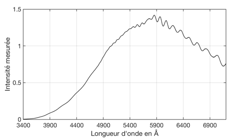
The spectral profile extracted is found at opposite. The signal is indeed weak in blue, maximum in the orange part, and we find our famous quantum efficiency oscillations (all the photonic sensors generate this kind of things, but in varying degrees).
At least for the visible wavelength, the spectral distribution of the radiation produced by a simple tungsten filament lamp, costing a few euros only, reveals extremely close to a black body radiation (a thermal emission). We will exploit this property.
ISIS offers a large number of tools that can be used from the command line (“Tools” tab, then “Commands”), the reason being not to overload the graphical interface. One of these commands is used to calculate the Planck profile of a black body from a temperature in Kelvin that is provided in parameters. This is the L_PLANCK command, so here is the syntax:
l_planck [file] [temperature] [lambda1] [Lambda2] [step]
with [file], the name of the Planck profile that the function will produce in the working directory in FITS format, [temperature], the black body temperature in Kelvin, [lambda1] and [lambda2], the wavelength limits from the product profile and [step], the wavelength step in the file.
Here I use a halogen lamp whose color temperature is given 2900 K by the manufacturer (in your purchases, look for a lamp with the highest color temperature possible for maximum signal in the blue). In my example, the parameters are:

After <return> the file “planck.fits” is produced with a step of 0.5 angstrom. Here is the spectral profile in question:

At this stage we have available on one side the measured spectrum of the lamp, which I call “lamp signal”, on the other side the spectral distribution in the light emitted by the lamp, the “black body profile”. The calculation of the instrument response is therefore trivial. It consists of dividing the first profile by the second:
“Instrument response” = “lamp signal” / “black body profile”
Note: this operation on two spectra can be done in ISIS several ways. For example, load the measured intensity profile of the lamp from the “Profile” tab and from the “Arithmetic” tool, fill in the “Divide by profile” field with the name “planck” and then “Apply”.
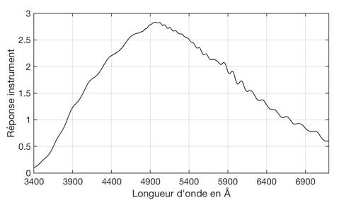
Here is the instrument response thus calculated:

The way to get this calibration file, which I will later call « direct_response” is very simple. I will show later, at the moment of exploiting it, that this result is quite honest.
It should be noted that this curve is the result of the product of optical transmission of the telescope, transmission of the spectrograph, the efficiency of the diffraction grating, the quantum efficiency of the detector (but not the atmosphere). It can be seen that the overall relative efficiency of the instrument is maximum around 5000 A, but remains high in the blue, which is a characteristic of the UVEX spectrograph (the decrease in UV is partly related to the RC mirror coatings). We also note the oscillations of the detector quantum efficiency, well present and therefore taken into account to correct the spectral data to be processed.
This “short” method is based entirely on the trust we know in the spectral distribution of the lamp But a halogen lamp of 2800K or 2900K produces a very insufficient number of photons to calibrate the UV part of the spectrum, which is a necessity with the UVEX spectrograph if we wish to exploit it in this part of the spectrum (it is not an obligation of course!). The « long » method will correct these difficulties.
But before addressing this second part, a note about accuracy of « response direct » evaluation…
Very often, the stray light produced by the optics of the spectrograph (scattering phenomenon on the components) produces a luminous background which potentially biases our result. The proof, in the parts of the image situated outside the zone illuminated by the slit, the signal is not strictly null. A bias (false zero) therefore potentially affects the calculated response profile. It can be corrected at least in part by considering “out of slit » areas with sky background areas. With this information, under ISIS, uncheck the box “Background sky not removed” in the “General” tab, then adjust the calculation areas of the sky background (“Calibration” tab) as shown in the screenshot below:

Then process the spectrum as before.
2. Long method
We will now use a light source which is a priori more reliable and produces a much whiter light than a tungsten lamp, or even a rather blue light. It will be the light coming from the stars themselves, and more particularly from the hot stars of A or B spectral type.
During an intermediate stage of the treatment we will also need the instrument response calculated during “short” method, the profile “direct_response”, and that does not pose very particular difficulties. So, the “long” method is actually a mixed method.
We use here the star Vega as a source of natural light, an A0V type object, whose spectral profile is well known (up to the UV, which is important when working with UVEX). Attention, it is necessary to observe with the minimal gain of a CMOS camera to put a long exposure regarding the atmospheric agitation, and also to average a large number of individual acquisitions. With a fixed gain CCD camera, an equivalent spectral type source (A or B) of lower brightness must be found in the MILES database for example. On the left, the apparent spectrum, without having applied instrument response correction, since considered unknown at this stage. This profile is called “vega_raw » (for example).

The next step is to temporarily divide the Vega star raw spectrum by the “direct_response” file. The latter is assimilated here to the pre-response of the instrument. The result is on the right, and it’s called “vega1” (this is an example). The performed operation is thus: “vega1” = “vega_raw » / “direct_response”. This work makes it possible to remove the « medium-frequency” variations from the apparent spectrum of the star, in particular here the oscillations of the quantum efficiency of the detector. This will make it possible to find the final instrument response more simply (note that the continuum is much smoother, except of course presence of Balmer lines).

The theoretical (or expected) spectrum of Vega is then recovered from the ISIS spectral database. I recommend the profile from the CALSPEC spectrophotometric base because it covers the ultraviolet, which is ideal for UVEX. This spectrum is called (see right) “vega_theoretical”. This is the true profile of the star outside the atmosphere, as we would like our instrument to restore it after data reduction in the ideal.

The next step is to divide the “vega1” spectrum by the “vega_theoretical” spectrum. The result is the spectrum that is called here “vega2”. The Balmer spectral lines theoretically must disappear. In this case, our spectrum UVEX is slightly more resolve than the CALSPEC database, also before the division, the UVEX spectrum is slightly degraded by filtering it with the tool “Filter” of “Profile” tab (convolution by a Gaussian function). The filtering parameter is found by successive tests so that in the “vega2” spectrum the residue of the Balmer lines is the least visible possible. The result is never perfect (the spectral line function of the instrument always produces distortions in the profile of the lines), but to do the best. It is also the moment to verify that the wavelength spectral calibration is correct (absence of marked local gradient effect, it is a severe test!).

The artifacts residual of the “vega2” profile are then erased by interactive smoothing with the help of the “Continuum” tool. Here again we need fingering for this operation, difficult to achieve otherwise than the hand. The goal is to eliminate the asperities that are obviously foreign to the instrumental response (asperities at the level of Balmer lines, telluric lines), while maintaining the low-frequency variations specific to the effective response. The result, named “vega3”, is shown at right.

The intermediate spectrum “vega3” is now multiplied by the file “direct_response” to take into account the « medium-frequency” characteristics of the instrument response (remember, in a previous step we divided by the file “direct_response” and here we do the opposite operation to return to the original situation somehow). The result spectrum is very close to the desired response (see right). It is called for the moment “vega4” and therefore, “vega4” = “vega3” x “direct_response”.

Take care, the “vega4” file is not yet the desired instrument response because some light energy of the star is lost through the atmosphere, and we have not considered until then. This prevents us from getting the pure instrument response at this stage (see the fundamental equation at the beginning of this article). To achieve this, we must compensate the effect of the atmosphere by calculating the spectral transmission in the direction of Vega star at the time of observation.
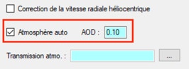
As is often the case in ISIS, there are several ways to perform this type of calculation. The “official” version first consists in finding the Vega star elevation above the horizon at the observation time from the “Heliocentric velocity » tab of the “Miscellaneous” tab. Here be careful to fill the fields “Longitude” and “Latitude” of the place of observation in the tab “Configuration”. Also use Universal Time to date your observations. The actual atmospheric transmission is then calculated from the “Miscellaneous” -> “Atmosphere” tab. The previously calculated angular elevation and an idea of AOD (horizontal transparency) must be provided. We are on May 13, 2019 during this observation, with a fairly clear night in a semi-urban, I adopted the value typical value for this period and situation, AOD = 0.1.
There is a trick to get faster to the atmospheric transmission using the processing of Vega spectrum:
From the “General” tab, tell ISIS to calculate the atmospheric transmission and apply it when processing the spectra. ISIS then searches for you the coordinates of the star in SIMBAD from the name you give in the “Object” field, then calculates the elevation and finally the transmission. Run the processing…

In the course of the operations, you notice that ISIS calculates the atmosphere transmission (at the time of the observation Vega was almost at the zenith — see angular elevation : 84,8 deg.).

The software produces in the working directory the file “atmo_Vega”: it is the atmospheric transmission. Everything is done automatically.

The atmospheric transmission calculated for an ADO of 0.1 (“atmo_Vega” file).
And here’s the finishing touch: dividing the “vega4” profile by the atmospheric transmission, we get the instrument response, as if it were operated outside the atmosphere, as if it were embedded on an artificial satellite. This is the real instrument response – see the curve at right It is called “inst_response”. So we made “reponse_inst” = “vega4” / “atmo_Vega”.
It is very instructive to compare the response found by the “short” method, by exploiting the single tungsten lamp, and the response found by the “long” method by exploiting the light of a star – see opposite. The difference is relatively small, which validates both methods. It is impressive to see the effectiveness of the “short” method in view of the simplicity of the means employed.

But for an accurate diagnosis of the quality of the one and other instrument response found, it is necessary to reduce the spectrum of our Vega star with the respective response curves. To do this, simply fill in the “Instrument response” field of the “General” tab with the name of the file of your choice (either “direct_response” or “inst_response”, see the example opposite). Of course, one must think of correcting the spectra of atmospheric transmission so that the calculated profile corresponds to an observation from space.

Tip: if you do not have an Internet connection or if the object is not found on SIMBAD, you can always calculate the atmospheric transmission by hand and give the result name in the field « Atmo. transmission »:

Be careful, you should NOT select “Automatic air mass” option. If you select this option, the atmospheric transmission to be supplied is that corresponding to a zenital transmission (“atmo_Vega_z0” for example).
The graphs below make it possible to compare the calculated Vega profile of the Vega in the two situations with the expected theoretical spectrum (MILES spectrum):


By processing with the response found via the “short method”, so without reference to any natural source, a discrepancy appears between the observed spectrum and the expected spectrum. This discrepancy is detrimental when performing precision spectrophotometric work, but the technical approach appears as a reasonable troubleshooting solution. Especially for users of UVEX, the analysis has been pushed up to 3250 A. In the UV, the situation is much more problematic. The fact that the tungsten lamp used produces almost no photon is paid down 3600 A.
Spectrum calculated using the “long method” response. This one sticks is very nearly similar to the theoretical spectrum. This is not surprising since we observe here the star that served as a reference. But we note that there is no significant error during operations (especially during the smoothing phase of the response file). The joint use of a natural and artificial standard source is effective. Note that the calculated response can potentially process spectra far in the ultraviolet.
3. Exploitation
An ultimate test is to use the previously measured instrument response, as well the atmospheric transmission calculation algorithm, to calibrate the spectrum of a star near the horizon line. I selected the star HD 175892 whose reference spectrum is available in the MILES database. At the time of observation, the star was close to the meridian, at an angular elevation of only 23.7 ° (air mass of 2.48). Atmospheric absorption is therefore severe. For proof, here is the comparison between the MILES spectrum and the observed spectrum without correction of the atmospheric transmission, where one notes a very large difference:

The usual logic would be to observe a nearby reference star in the sky to evaluate a new adapted “instrument response” (a local response somehow). But we have taken care here to calculate an intrinsic response to the instrument, independent of the atmosphere transmission… The spectrum is finally reduced with the universal file “response_inst” and asking ISIS to automatically evaluate the atmospheric transmission (AOD = 0.1 and select automatic option). Here the result:

Without this being perfect (it can never be!) the calculated profile is very close to the theoretical spectrum, whereas the conditions are quite extreme (low star on the horizon). This confirms the universal nature of the calculated instrument response, and also the efficiency of the atmospheric transmission model employed, and more generally, of the processing procedure. At this point, if a significant gap were noticeable, it could be attributed to a wrong AOD choice: if necessary test a new value, which is immediate with the automatic function of ISIS, then to check if the difference is reduced (in case of doubt, it is also a technique to find at the beginning of observation for example the good ADO for the night, by observing a low star).
Be careful concerning atmospheric differential refraction during verification and exploitation: a good result can only be obtained if the star is close to the meridian, or when the axis of the slit is oriented according to the parallactic angle, for example by a voluntary rotation of the spectrograph, or using an ADC system suitable for spectrography (see note at the beginning of the article), or modeling the effect. Of course, the problem of the differential refraction fades as we observe the stars at a high angular height compared to the horizon.
In the acquisition conditions presented, the HD 175892 observed spectrum proves to be very well radiometrically calibrated whereas we did not need to calculate a specific instrument response for the situation, as the “response_inst” reference file could very well have been generated several weeks before the said observation. One guesses the productivity gain and the simplification of the life of the observer that this represents.
Complement. During this demonstration, I never filled the “Flat” item of the “General” tab:

What happens if we fill this item? During preprocessing, ISIS subtracts the offset, the dark, AND then divides by the specified flat-field image, for example the image “flat_2D” (see at the beginning of the article). This is a priori the “official” procedure. Ideally, it allows in particular to eliminate the shadow of dusts present in the optical path, or to correct the gain variation from pixel to pixel (this latter concerns the “high-frequency” (HF) variation of the instrument response). It is preferred here to ignore the dust traces and the PRNU (Pixel Response Non Uniformity) : it is assumed that the system is clean, free of dust – a credible hypothesis if you are careful, and that the PRNU is of low value (of the order of 1%) to make it negligible compared to other sources of response error. The problem of dividing by the “flat_2D” image is that one becomes very sensitive to the evolutions of the instrument setting, mechanical flexure and non-uniform illumination of the telescope entrance pupil (variation of the apparent F/D compared to the observation, which can change the projected position of dust shadows). If the “flat_2D” image does not coincide geometrically to the image to be processed, the cure may be worse than the harm if we want to eliminate the dust trace, for example. Also, although it is not ideal and complete, I recommend to follow rather the processing method of this demonstration, safer and faster.
If you still want process a PRNU problem or interference fringes problem, without changing the flow presented in this article, I propose to isolate the HF component of the flat-field with a specific ISIS tool (“Masters” tab) :

Here is the characteristic aspect of the “flat_2D_HF” image thus produced:
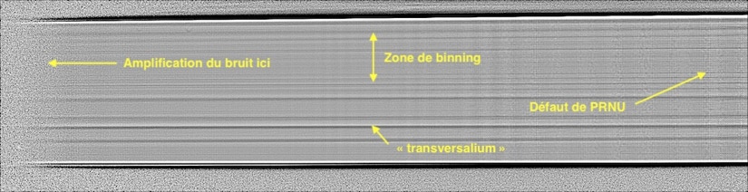
PRNU defects are well taken into account in this new calibration image, but beware, in the parts where the flat-field image is not very intense (in the blue with a halogen lamp) the division will amplify the noise, this is a significant disadvantage. However, if you want to use such an image because your spectra are suitable or you see a big problem, do the processing by following the “pipeline” of this article, but add:

Conclusion. I presented here with some details my own procedure for reduce low and medium resolution spectrums. The end result is that the time spent finding the real response from the « long version » algorithm (better because more rigorous and necessary with UVEX) actually only represents a brief moment. The spectra acquisition and processing is greatly facilitated and the quality improved. The next step is to add a descent atmospheric chromatic correction solution for the future. In addition, unfolding this procedure (a “pipeline”) in a strict way allows to better to know his equipment and better use it eventually.